Mastering INDEX and MATCH: A Powerful Alternative to VLOOKUP

Introduction

In Excel, being able to pull and organize data efficiently can be very useful. Many users rely on VLOOKUP for this, but combining INDEX and MATCH gives you more flexibility. This article explains how both functions work, their advantages, and how to apply them.

The INDEX Function

The INDEX function returns a value from a specific position in a range.

The syntax is:

=INDEX(array, row_num, [column_num])

• array: The range of cells to search.
• row_num: The row number to return from the range.
• column_num: (Optional) The column number to return from. If omitted, it defaults to the first column.

The MATCH Function

The MATCH function finds the position of a value in a range.

The syntax is:

=MATCH(lookup_value, lookup_array, [match_type])

• lookup_value: The value to look for.
• lookup_array: The range of cells to search.
• match_type: (Optional)
  • 0 = exact match
  • 1 = largest value less than or equal to the lookup_value (ascending order)
  • -1 = smallest value greater than or equal to the lookup_value (descending order)

Why Use INDEX and MATCH Instead of VLOOKUP?

• Works in any direction: VLOOKUP can only look to the right, but INDEX and MATCH can return values from the left or right.
• Dynamic column references: VLOOKUP requires hard-coded column numbers that break when columns are added or removed. INDEX and MATCH adjust more easily.
• Better for large datasets: INDEX and MATCH often calculate faster because they don't force Excel to scan entire tables for every lookup.
• No sorting required: VLOOKUP can give errors if data isn't sorted (when using approximate match). INDEX and MATCH return correct results regardless of order.

How to Use INDEX and MATCH Together

To effectively use INDEX and MATCH in tandem, follow these steps:

Step 1: Setting Up Your Data

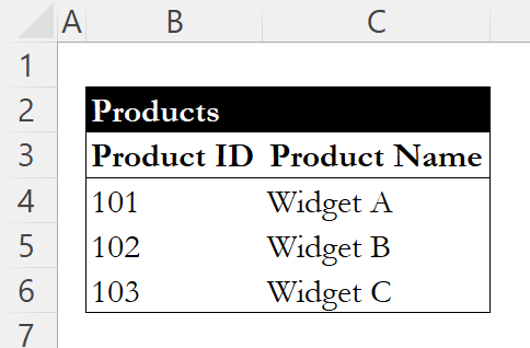
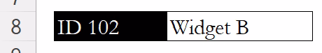
Consider a dataset with two columns: Product ID and Product Name. For instance:

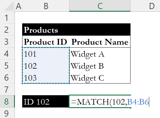
Step 2: Using MATCH to Find the Row Number

Suppose you want to find the Product Name for Product ID 102. First, use the MATCH function to identify the row number of Product ID 102:

=MATCH(102, B4:B6, 0)

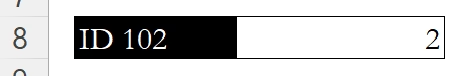
This function returns 2, as Product ID 102 is the second item in the range.

Step 3: Using INDEX to Retrieve the Product Name

Now, use the INDEX function combined with MATCH to get the corresponding Product Name:

=INDEX(C4:C6, MATCH(102, B4:B6, 0))

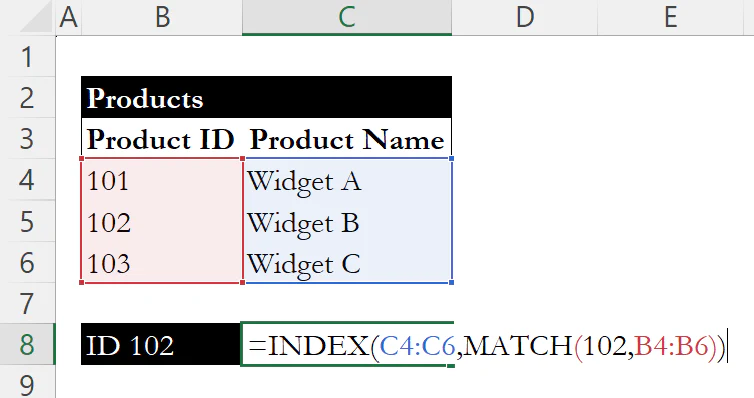
This formula returns "Widget B", as it pulls the value from the second row of the Product Name column.

Conclusion

Using INDEX and MATCH together is a flexible way to look up data in Excel. Unlike VLOOKUP, it works in any direction and adapts better when your data changes. Learning this approach can make everyday lookups more reliable and easier to maintain.

If you're looking for a newer alternative, check out our guide on XLOOKUP for a streamlined lookup function that combines the best of both worlds. For a side-by-side comparison of the traditional approach and its modern replacement, see VLOOKUP vs. XLOOKUP.