How to Use XLOOKUP in Excel (With Examples)

Introduction

Excel's XLOOKUP function makes it easy to pull related information from different tables. Imagine you're analyzing clothing sales. In one sheet, you only see the sales value linked to an item ID. In another sheet, that same item ID is tied to the buyer's gender. By using XLOOKUP, you can bring the gender data directly into your sales table. Once it's there, you can quickly filter and compare sales by gender without manually cross-checking IDs.

What is XLOOKUP?

XLOOKUP searches for a value in one column (or array) and returns a related value from another. It replaces older functions like VLOOKUP and HLOOKUP with a simpler, more flexible syntax.

The syntax is:

=XLOOKUP(lookup_value, lookup_array, return_array, [if_not_found])

• lookup_value: The value you want to search for.
• lookup_array: The range where Excel should look for that value.
• return_array: The range that contains the value to return.
• [if_not_found]: Optional message or value if no match is found.

XLOOKUP in Action

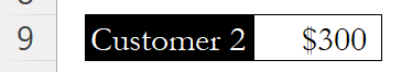
Suppose you have the following sales data:

If you want to know how much Customer 2 spent, enter:

=XLOOKUP("Customer 2", B4:B7, C4:C7)

Excel searches column B for "Customer 2" and returns the corresponding amount from column C: $300.

Handling Missing Data

If the name isn't in the list, you can prevent an error by adding a custom message. For example:

=XLOOKUP("Customer 73", B4:B7, C4:C7, "Not Found")

If "Customer 73" isn't listed, Excel will display "Not Found" instead of an error.

Conclusion

XLOOKUP combines the flexibility of older lookup functions into one. With it, you can quickly connect datasets, handle missing values gracefully, and save time when analyzing data.

Once your data is in one place, you can use COUNTIF and SUMIF to count and sum values based on conditions.