How to Use the FILTER Function in Excel

Introduction

The FILTER function extracts data from a range based on criteria you define. It updates automatically if the source data changes, making it more flexible than copying and pasting or applying filters through the ribbon.

Filter Function Syntax

The syntax is:

=FILTER(array, include, [if_empty])

• array: The range of cells to filter.
• include: The condition that decides which rows or columns are returned.
• [if_empty]: An optional result if no data matches.

Filter Function Example

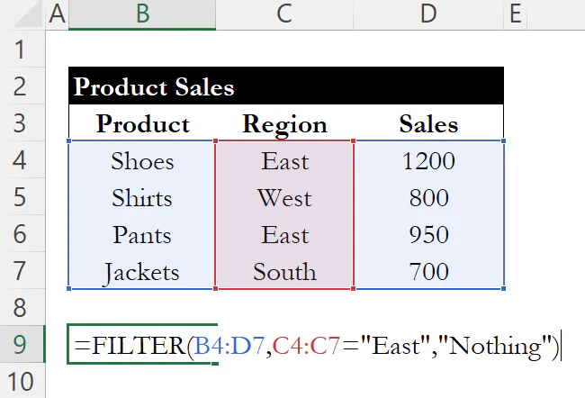
Suppose you have a dataset of products, regions, and sales values in columns B–D. To return only the rows where the region is East, enter:

=FILTER(B4:D7, C4:C7="East", "Nothing")

The result will be:

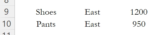
If no rows matched, the formula would return "Nothing."

Why Use FILTER in Excel

FILTER removes the need for manual steps when narrowing down data. It makes reports cleaner and ensures that outputs update automatically as the underlying dataset changes.

Conclusion

The FILTER function is a straightforward way to extract only the data you need. By applying conditions directly in the formula, you can keep your spreadsheets both accurate and easy to interpret.

If you need to pull a single value from another table, check out our guide on INDEX and MATCH for flexible data lookups. To arrange your filtered results, see how to use SORT and SORTBY.